Asthma and heart disease in NY state

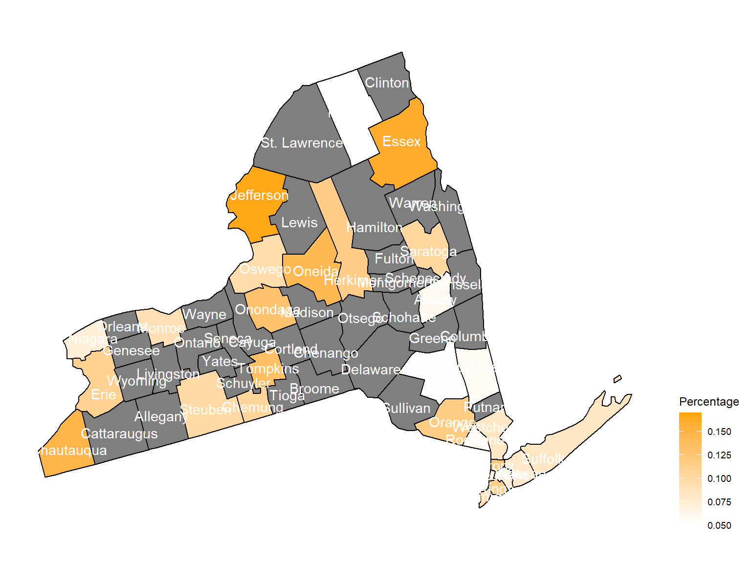
• Considering geological factor as an important predictor, we calculated percentage of asthma cases based on their locations with respect to counties in NY state and created maps with their asthma rate based on colors among counties in NY state.If the color is grey, that means there was no respondents in those counties at that year.

Asthma Map

According to the graphs, we can know that:

• In 2003, Chautauqua county is with the most asthma patients. After that, the percentage decreased until 2009.
• After 2008, asthma patients in Steuben and Chemung were increasing.
• Counties in north of New York, including Jefferson, St. Lawrence, Franklin and Essex are also with higher percentage of asthma patients.
• Urban counties, including Bronx, Queens and Erie, are also with a higher percentage of asthma patients.

2003

asthma_now_county_df1 = 
  brfss_air_df %>% 
  mutate(
    fips = str_c(state_code.x,county_code)
  ) %>% 
  group_by(state_code.x, county_code,county,fips, year) %>% 
  filter(year == 2003) %>% 
  count(
    county,asthma_status
  ) %>% 
  mutate(
    percent = n/sum(n)
  ) %>% 
  filter(asthma_status == "1") %>% 
  spread(asthma_status, percent)

asthma_now_county_plot_map = 
  plot_usmap(regions = "county", include = c("NY"), data = asthma_now_county_df1, values = "1", label = TRUE, label_color = "White") +
  scale_fill_continuous(
    low = "white", high = "Orange", name = "Percentage", label = scales::comma, limits = c(0.05,0.17)
  ) + 
  theme(legend.position = "right")

asthma_now_county_plot_map

2004

asthma_now_county_df2 = 
  brfss_air_df %>% 
  mutate(
    fips = str_c(state_code.x,county_code)
  ) %>% 
  group_by(state_code.x, county_code,county,fips, year) %>% 
  filter(year == 2004) %>% 
  count(
    county,asthma_status
  ) %>% 
  mutate(
    percent = n/sum(n)
  ) %>% 
  filter(asthma_status == "1") %>% 
  spread(asthma_status, percent)

asthma_now_county_plot_map = 
  plot_usmap(regions = "county", include = c("NY"), data = asthma_now_county_df2, values = "1", label = TRUE, label_color = "White") +
  scale_fill_continuous(
    low = "white", high = "Orange", name = "Percentage", label = scales::comma, limits = c(0.05,0.17)
  ) + 
  theme(legend.position = "right")

asthma_now_county_plot_map

2005

asthma_now_county_df3 = 
  brfss_air_df %>% 
  mutate(
    fips = str_c(state_code.x,county_code)
  ) %>% 
  group_by(state_code.x, county_code,county,fips, year) %>% 
  filter(year == 2005) %>% 
  count(
    county,asthma_status
  ) %>% 
  mutate(
    percent = n/sum(n)
  ) %>% 
  filter(asthma_status == "1") %>% 
  spread(asthma_status, percent)

asthma_now_county_plot_map = 
  plot_usmap(regions = "county", include = c("NY"), data = asthma_now_county_df3, values = "1", label = TRUE, label_color = "White") +
  scale_fill_continuous(
    low = "white", high = "Orange", name = "Percentage", label = scales::comma, limits = c(0.05,0.17)
  ) + 
  theme(legend.position = "right")

asthma_now_county_plot_map

2006

asthma_now_county_df4 = 
  brfss_air_df %>% 
  mutate(
    fips = str_c(state_code.x,county_code)
  ) %>% 
  group_by(state_code.x, county_code,county,fips, year) %>% 
  filter(year == 2006) %>% 
  count(
    county,asthma_status
  ) %>% 
  mutate(
    percent = n/sum(n)
  ) %>% 
  filter(asthma_status == "1") %>% 
  spread(asthma_status, percent)

asthma_now_county_plot_map = 
  plot_usmap(regions = "county", include = c("NY"), data = asthma_now_county_df4, values = "1", label = TRUE, label_color = "White") +
  scale_fill_continuous(
    low = "white", high = "Orange", name = "Percentage", label = scales::comma, limits = c(0.05,0.17)
  ) + 
  theme(legend.position = "right")

asthma_now_county_plot_map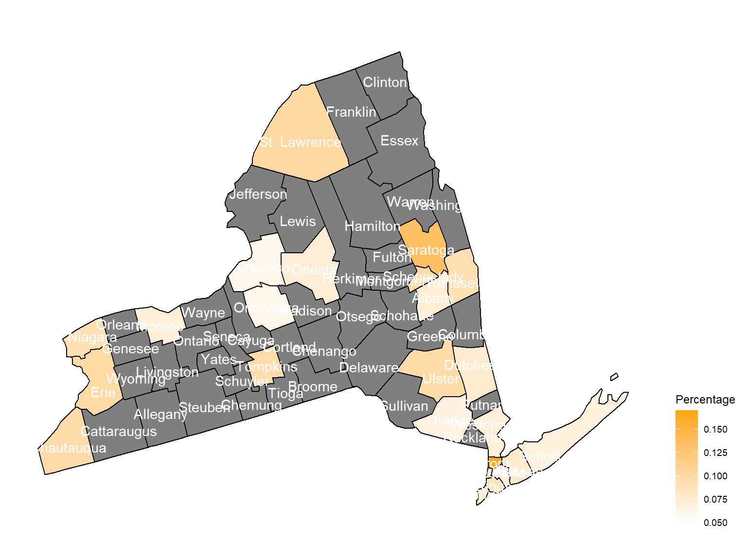

2007

asthma_now_county_df5 = 
  brfss_air_df %>% 
  mutate(
    fips = str_c(state_code.x,county_code)
  ) %>% 
  group_by(state_code.x, county_code,county,fips, year) %>% 
  filter(year == 2007) %>% 
  count(
    county,asthma_status
  ) %>% 
  mutate(
    percent = n/sum(n)
  ) %>% 
  filter(asthma_status == "1") %>% 
  spread(asthma_status, percent)

asthma_now_county_plot_map = 
  plot_usmap(regions = "county", include = c("NY"), data = asthma_now_county_df5, values = "1", label = TRUE, label_color = "White") +
  scale_fill_continuous(
    low = "white", high = "Orange", name = "Percentage", label = scales::comma, limits = c(0.05,0.17)
  ) + 
  theme(legend.position = "right")

asthma_now_county_plot_map

2008

asthma_now_county_df6 = 
  brfss_air_df %>% 
  mutate(
    fips = str_c(state_code.x,county_code)
  ) %>% 
  group_by(state_code.x, county_code,county,fips, year) %>% 
  filter(year == 2008) %>% 
  count(
    county,asthma_status
  ) %>% 
  mutate(
    percent = n/sum(n)
  ) %>% 
  filter(asthma_status == "1") %>% 
  spread(asthma_status, percent)

asthma_now_county_plot_map = 
  plot_usmap(regions = "county", include = c("NY"), data = asthma_now_county_df6, values = "1", label = TRUE, label_color = "White") +
  scale_fill_continuous(
    low = "white", high = "Orange", name = "Percentage", label = scales::comma, limits = c(0.05,0.17)
  ) + 
  theme(legend.position = "right")

asthma_now_county_plot_map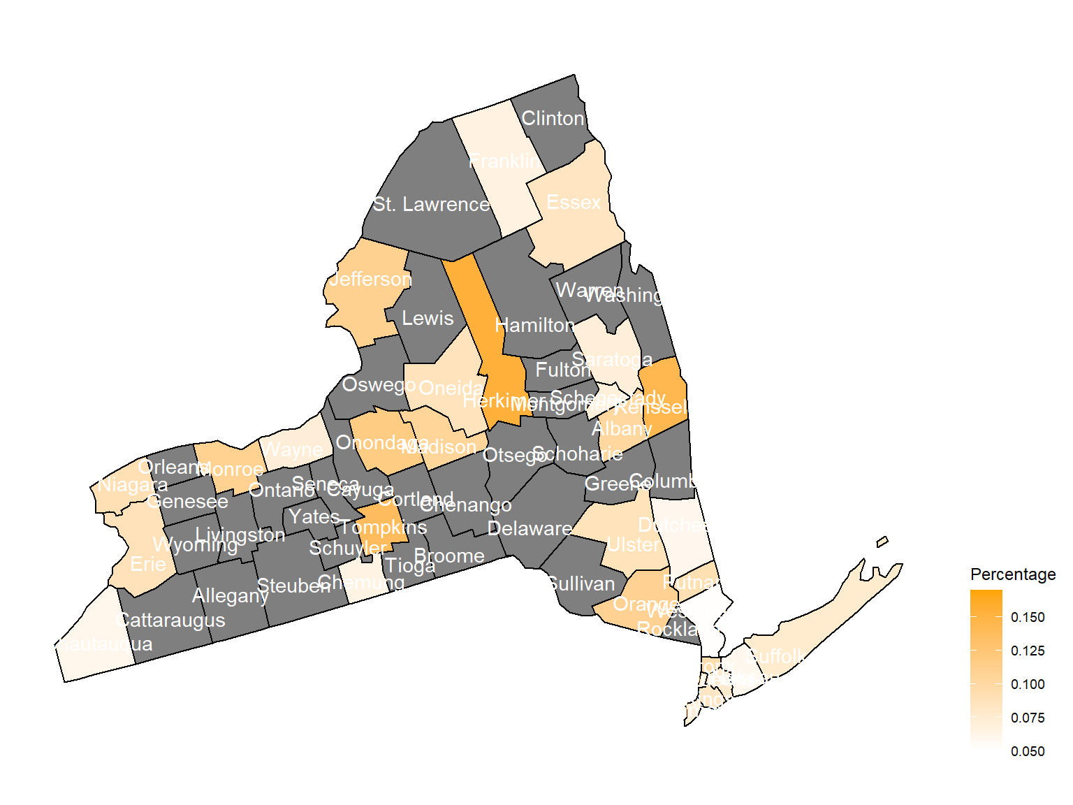

2009

asthma_now_county_df7 = 
  brfss_air_df %>% 
  mutate(
    fips = str_c(state_code.x,county_code)
  ) %>% 
  group_by(state_code.x, county_code,county,fips, year) %>% 
  filter(year == 2009) %>% 
  count(
    county,asthma_status
  ) %>% 
  mutate(
    percent = n/sum(n)
  ) %>% 
  filter(asthma_status == "1") %>% 
  spread(asthma_status, percent)

asthma_now_county_plot_map = 
  plot_usmap(regions = "county", include = c("NY"), data = asthma_now_county_df7, values = "1", label = TRUE, label_color = "White") +
  scale_fill_continuous(
    low = "white", high = "Orange", name = "Percentage", label = scales::comma, limits = c(0.05,0.17)
  ) + 
  theme(legend.position = "right")

asthma_now_county_plot_map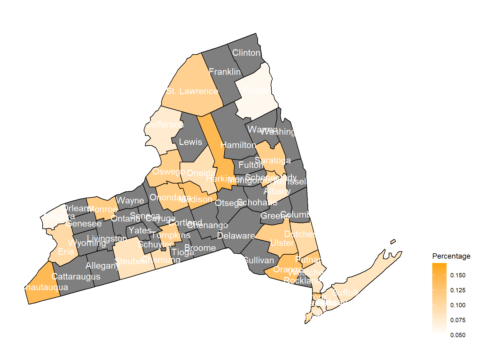

2010

asthma_now_county_df8 = 
  brfss_air_df %>% 
  mutate(
    fips = str_c(state_code.x,county_code)
  ) %>% 
  group_by(state_code.x, county_code,county,fips, year) %>% 
  filter(year == 2010) %>% 
  count(
    county,asthma_status
  ) %>% 
  mutate(
    percent = n/sum(n)
  ) %>% 
  filter(asthma_status == "1") %>% 
  spread(asthma_status, percent)

asthma_now_county_plot_map = 
  plot_usmap(regions = "county", include = c("NY"), data = asthma_now_county_df8, values = "1", label = TRUE, label_color = "White") +
  scale_fill_continuous(
    low = "white", high = "Orange", name = "Percentage", label = scales::comma, limits = c(0.05,0.17)
  ) + 
  theme(legend.position = "right")

asthma_now_county_plot_map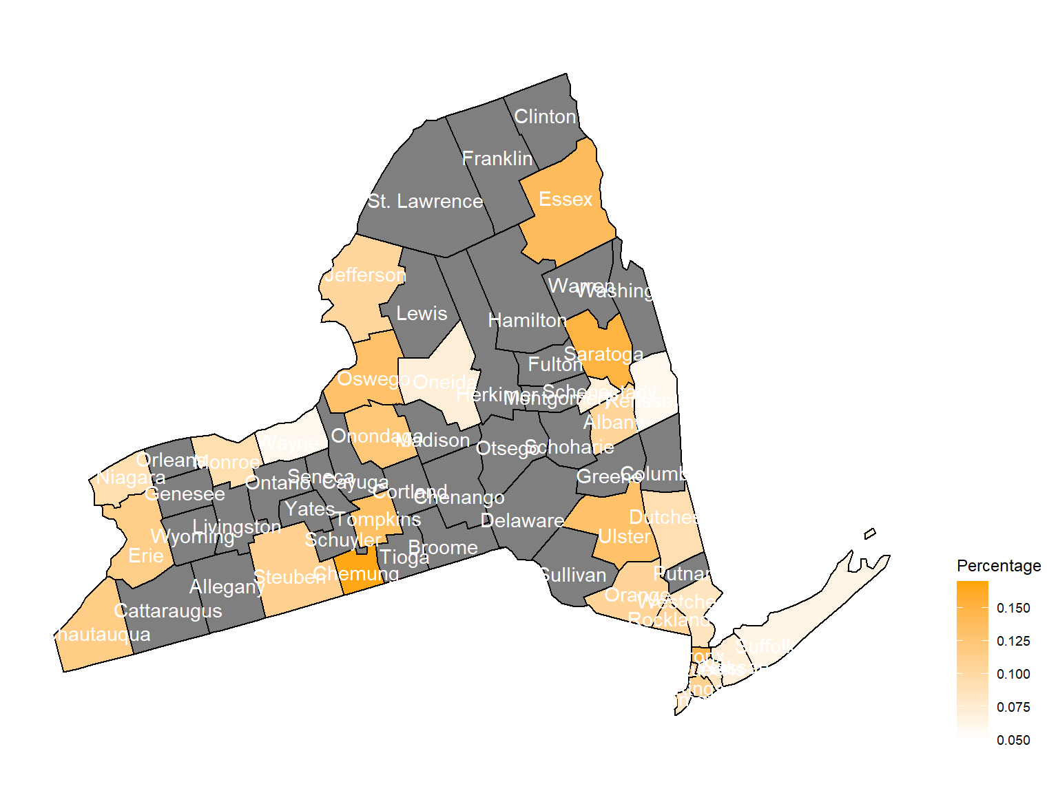

2011

asthma_now_county_df9 = 
  brfss_air_df %>% 
  mutate(
    fips = str_c(state_code.x,county_code)
  ) %>% 
  group_by(state_code.x, county_code,county,fips, year) %>% 
  filter(year == 2011) %>% 
  count(
    county,asthma_status
  ) %>% 
  mutate(
    percent = n/sum(n)
  ) %>% 
  filter(asthma_status == "1") %>% 
  spread(asthma_status, percent)

asthma_now_county_plot_map = 
  plot_usmap(regions = "county", include = c("NY"), data = asthma_now_county_df9, values = "1", label = TRUE, label_color = "White") +
  scale_fill_continuous(
    low = "white", high = "Orange", name = "Percentage", label = scales::comma, limits = c(0.05,0.17)
  ) + 
  theme(legend.position = "right")

asthma_now_county_plot_map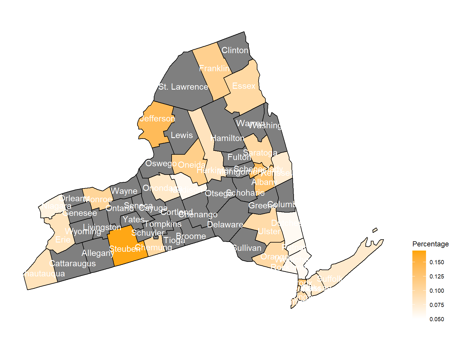

2012

asthma_now_county_df10 = 
  brfss_air_df %>% 
  mutate(
    fips = str_c(state_code.x,county_code)
  ) %>% 
  group_by(state_code.x, county_code,county,fips, year) %>% 
  filter(year == 2012) %>% 
  count(
    county,asthma_status
  ) %>% 
  mutate(
    percent = n/sum(n)
  ) %>% 
  filter(asthma_status == "1") %>% 
  spread(asthma_status, percent)

asthma_now_county_plot_map = 
  plot_usmap(regions = "county", include = c("NY"), data = asthma_now_county_df10, values = "1", label = TRUE, label_color = "White") +
  scale_fill_continuous(
    low = "white", high = "Orange", name = "Percentage", label = scales::comma, limits = c(0.05,0.17)
  ) + 
  theme(legend.position = "right")

asthma_now_county_plot_map